Recruitment Data Transformation and Analysis
Integrated 800k+ job postings from 3 sources into unified optimized Power BI report
Project Overview
Transformed fragmented recruitment data from multiple sources into a standardized schema, implementing automated data ingestion and optimized Power BI visualizations for strategic workforce planning.
Client Requirements
- Data Tables into Database: Loaded different data tables format from a folder into a database
- Data Consolidation: Merge normalized/centralized data from 3 sources
- Schema Standardization: Create unified table with 12-column structure
- Performance Optimization: Handle 800k+ rows efficiently
- Trend Analysis: 6 key analytical requirements for hiring insights
View Task Email
Data Tables
| Source 1 | Source 2 | Source 3 |
|---|---|---|
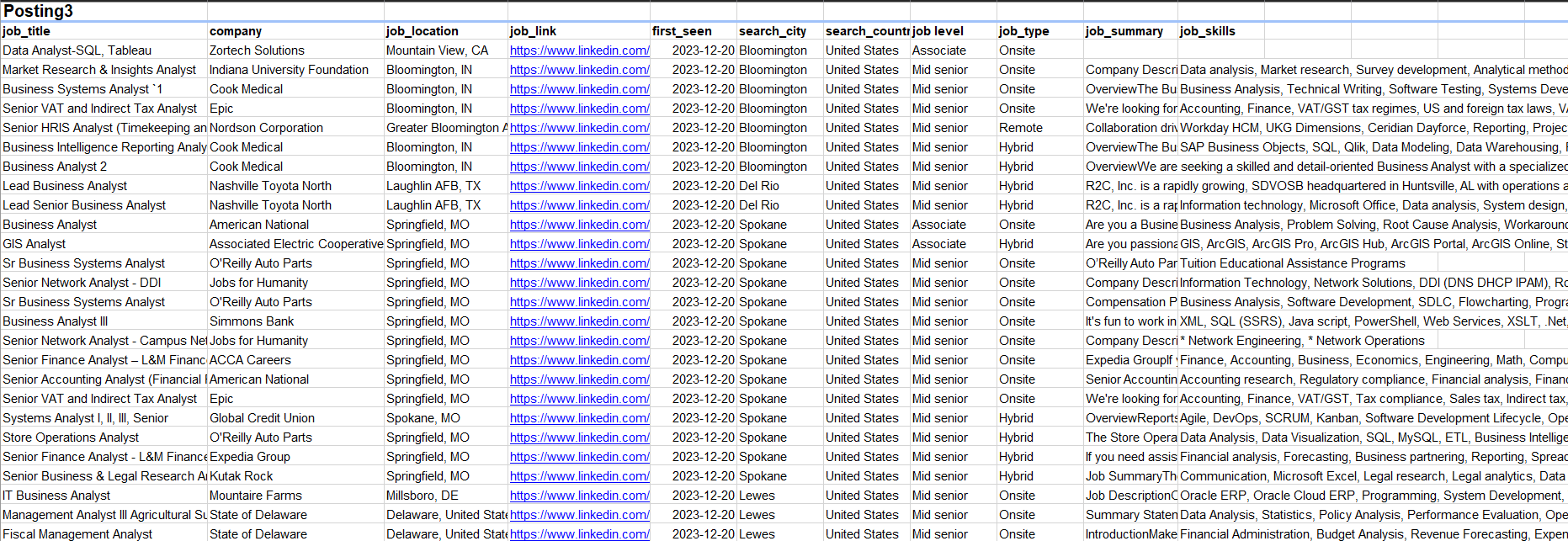
| Job_posting1 (Fact Table) | Job_postings_facts2 (Fact Table) | Posting3 |
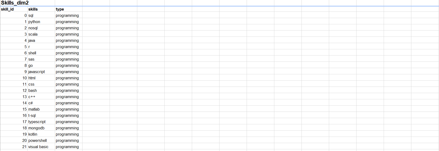
| Job_skills1 (Dimension Table) | Skills_dim2 (Dimension Table) | |
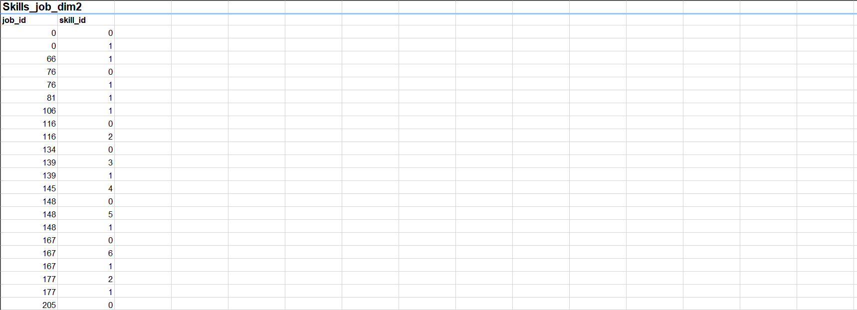
| Job_summar1 (Dimension Table) | Skills_job_dim2 (Dimension Table) | |
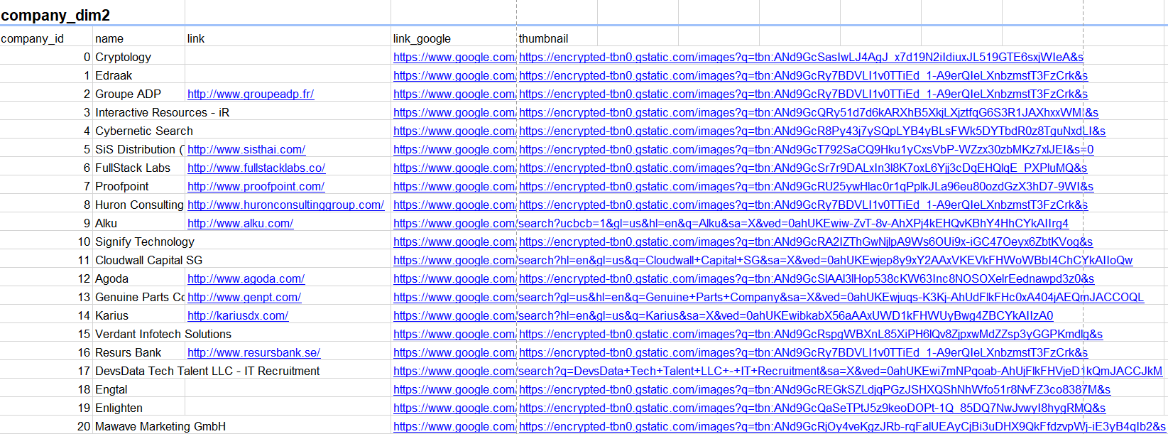
| Company_dim2 (Dimension Table) |
Implementation Steps
1. Automated Database Loading
Automatically loaded all data files from a local folder into the MySQL bidb database.
- Connected using SQLAlchemy’s
create_engine. - Detected file type and target table name from each filename.
- Read files using:
pd.read_excelfor.xlsxpd.read_csvfor.csvpd.read_jsonfor others
- Loaded data into MySQL with
df.to_sql(...) - Displayed progress after each table was loaded.
Python Data Ingestion Script
# create connection with destination database
# read data file path
# extract the name of table and data format
# load it into database with same data table name

engine = create_engine('mysql+pymysql://root:1234@localhost/bidb')

for filepath in glob.glob(r'C:\Users\aly98\Desktop\Power BI\Projects\HR\Data/*'):
    table_name = filepath.split(sep='\\',maxsplit=-1)[-1].split('.')[0]
    data_format = filepath.split(sep='\\',maxsplit=-1)[-1].split('.')[1]

    if data_format == 'xlsx':
        df = pd.read_excel(filepath)
    elif data_format == 'csv':
        df  = pd.read_csv(filepath)
    else:
        df = pd.read_json(filepath)

    df.to_sql(name = table_name, con=engine, if_exists='replace', index=False, chunksize=10000, method='multi')
    print(f'{table_name} table loaded')
2. Data Loading and Transformation in Power BI
Transformation in Power Query
Sources Used
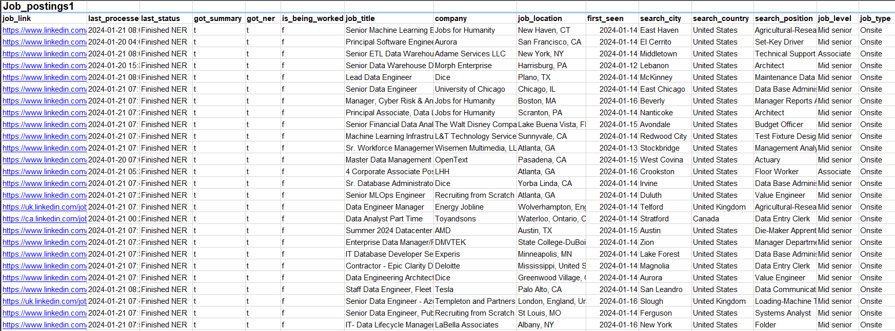
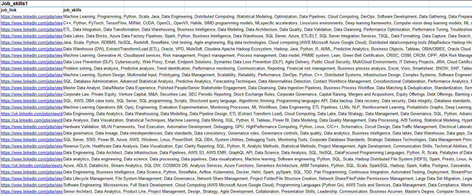
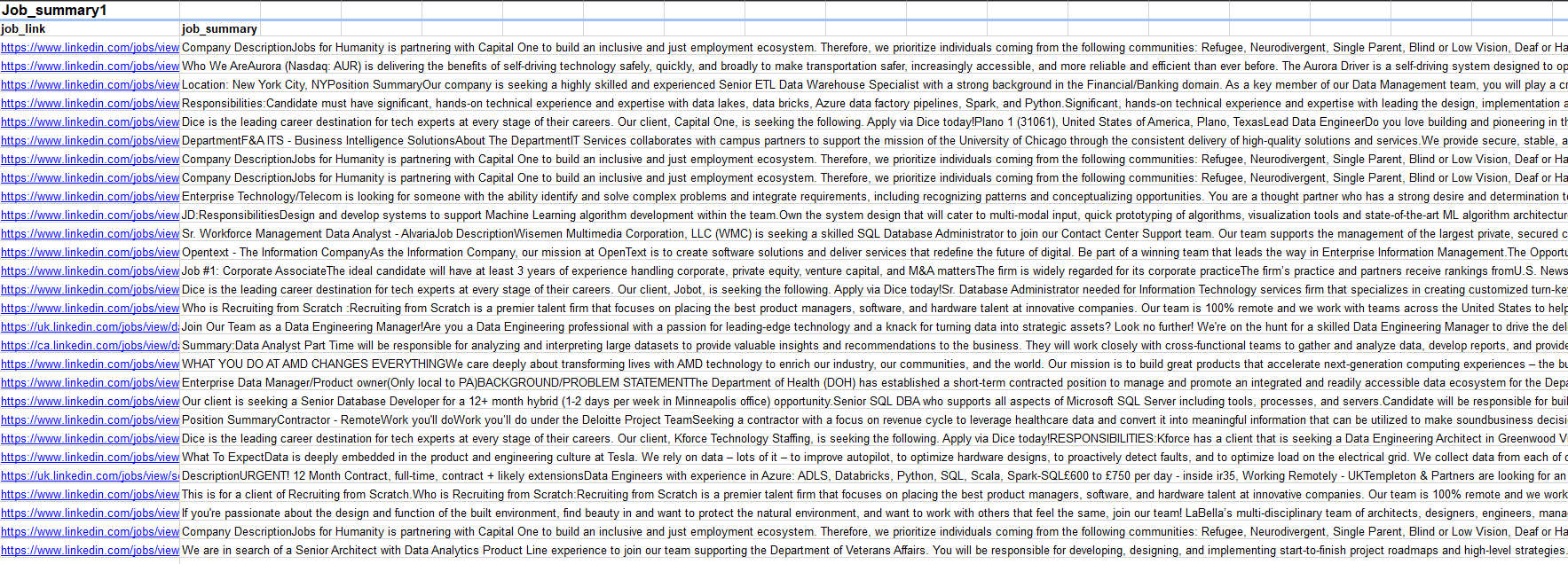
- Source 1: job_postings1, job_skills1, job_summary1
- Source 3: posting3
Cleaned and merged Source 1 tables in Power BI using Power Query, considering the client's desired schema. Here, job_postings1 is treated as the fact table, while job_skills1 and job_summary1 are dimension tables.
- Removed irrelevant columns from
job_postings1. - Renamed columns for consistency.
- Extracted
Job_idfrom job URL. - Merged
job_skills1intojob_postings1to include skills. - Merged
job_summary1intojob_postings1to include summaries. - Converted columns to appropriate data types.
Source 3: Transformation
- Renamed columns to match Source 1 structure.
- Removed irrelevant columns.
- Converted data types appropriately.
- Extracted
Job_id.
Appended Source 3 (posting3) to the cleaned Source 1 dataset to create a unified dataset.
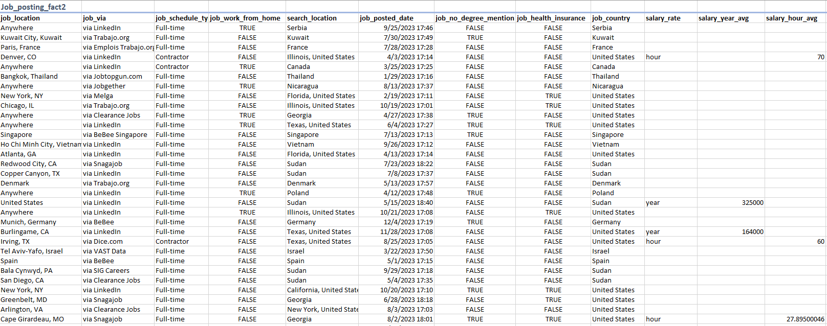
Source 2: Transformation with Python
Used Python to reshape and aggregate Source 2 data due to many-to-one relationships (multiple skills per job_id), which could not be handled effectively in Power Query.
Python script
from sqlalchemy import create_engine
import pandas as pd

engine = create_engine('mysql+pymysql://root:1234@localhost/bidb')

company = pd.read_sql("SELECT * FROM company_dim2", con=engine)
job_post = pd.read_sql("SELECT * FROM job_postings_fact2", con=engine)
skill = pd.read_sql("SELECT * FROM skills_dim2", con=engine)
skill_job = pd.read_sql("SELECT * FROM skills_job_dim2", con=engine)

df = skill_job.merge(skill, on='skill_id', how='left')
skills_table = df.groupby('job_id')['skills'].agg(','.join).reset_index()

job_post = job_post.merge(company, on='company_id', how='left')
job_post = job_post.merge(skills_table, on='job_id', how='left')

job_post.drop(columns=['job_via', 'search_location', 'job_no_degree_mention', 'job_health_insurance',
                       'salary_rate', 'salary_year_avg', 'salary_hour_avg', 'link', 'link_google',
                       'thumbnail', 'company_id'], inplace=True)

job_post.rename(columns={
    'job_title_short': 'Job_field',
    'job_title': 'Job_title',
    'job_schedule_type': 'Job_employment_type',
    'job_work_from_home': 'Job_type',
    'job_posted_date': 'Job_posting_date',
    'job_country': 'Country',
    'name': 'Company_name',
    'skills': 'Job_skills',
    'job_id': 'Job_id'
}, inplace=True)
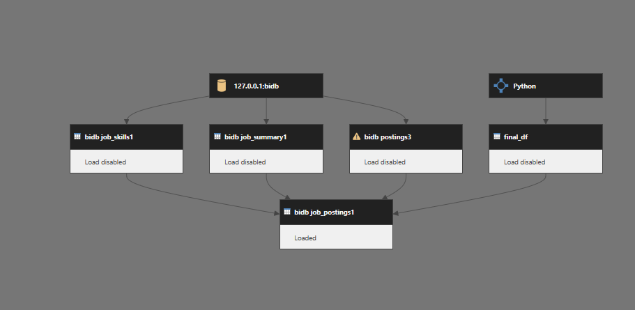
The final DataFrame was loaded into Power BI as a separate data source.
Post-Load Processing in Power BI
After loading Source 2 into Power BI, added a derived column to classify job type:
= Table.AddColumn(job_post1, "Job_type", each if [job_work_from_home] = "1" then "remote" else "onsite")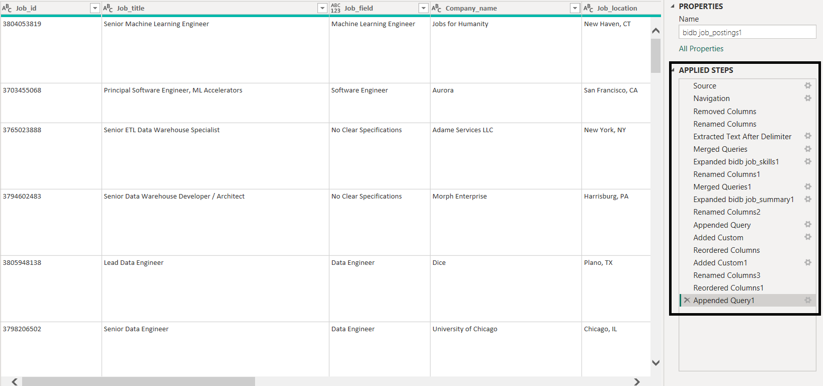
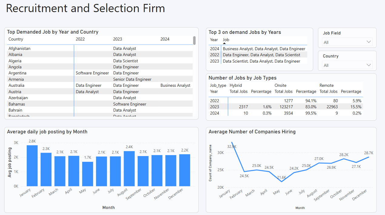
3. Power BI Visualizations and Business Insights
1. Average Daily Job Openings
The company faced difficulties identifying hiring trends over time, affecting strategic workforce planning. To address this, a bar chart was implemented using a DAX measure that calculates the average number of job postings per day per month.
Avg job posting =
VAR selected_month = SELECTEDVALUE('bidb job_postings1'[Job_posting_date].[Month])
VAR total_days = CALCULATE(DISTINCTCOUNT('bidb job_postings1'[Job_posting_date].[Date]),
                           FILTER('bidb job_postings1',
                                  'bidb job_postings1'[Job_posting_date].[Month] = selected_month))
VAR total_openings = COUNT('bidb job_postings1'[Job_id])
RETURN total_openings / total_days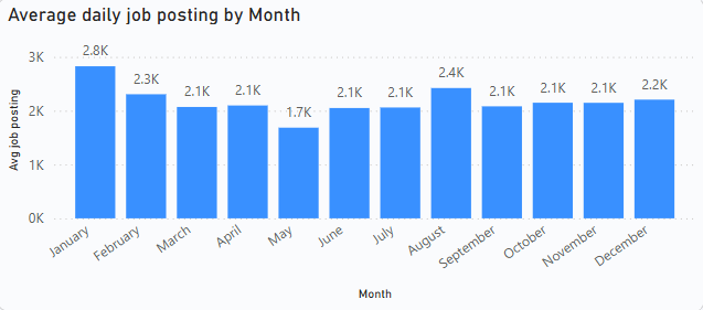
Insight: The average daily job postings are highest in January and August, indicating peak hiring periods. Conversely, the lowest hiring activity occurs in May. Other months show relatively stable hiring trends with minimal fluctuations.
2. Job Type Distribution Over the Years
To analyse the distribution of onsite and remote jobs across years, a table visualization was created. It shows the total number of companies offering each job type and their contribution percentages. This analysis informs better strategic recruitment planning.
Measures used:
Total_company =
SUMX(VALUES('bidb job_postings1'[Job_type]),
     CALCULATE(DISTINCTCOUNT('bidb job_postings1'[Company_name])))
job_Contribution_Years =
VAR total_job = CALCULATE([Total_company], ALL('bidb job_postings1'[Job_type]))
RETURN [Total_company] / total_job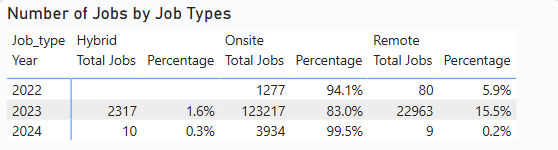
Insight: Onsite jobs consistently dominated across all years, accounting for over 90% of postings, except in 2023 where they slightly declined to 83%. Remote jobs started at 5.9% in 2022, increased to nearly 10% in 2023, and then dropped to less than 1% in 2024. Hybrid roles remained minimal throughout — nearly nonexistent in 2022, 1.6% in 2023, and less than 1% in 2024.
Note: The data volume for 2022 and 2023 is relatively low, so insights from these years may not be fully reliable.
3. Dominant Job Types by Country and Year
A matrix table was used to identify the most frequent job fields for each country and year. This helps tailor recruitment strategies to local demands and global trends.
Popular_Job_Year =
VAR selected_country = SELECTEDVALUE('bidb job_postings1'[Country])
VAR selected_year = SELECTEDVALUE('bidb job_postings1'[Job_posting_date].[Year])
VAR job_occurance =
    SUMMARIZE(
        FILTER('bidb job_postings1',
               'bidb job_postings1'[Country] = selected_country &&
               'bidb job_postings1'[Job_posting_date].[Year] = selected_year &&
               'bidb job_postings1'[Job_field] <> "No Clear Specifications"),
        'bidb job_postings1'[Job_field],
        "job_field_count", COUNT('bidb job_postings1'[Job_field])
    )
VAR max_posting = MAXX(job_occurance, [job_field_count])
RETURN MAXX(FILTER(job_occurance, [job_field_count] = max_posting), 'bidb job_postings1'[Job_field])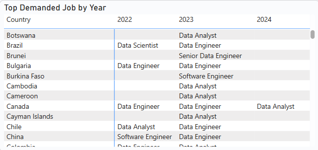
Insight: For your complete data refer to the Power BI report
4. Monthly Hiring Activity
To gauge market stability and activity, a line chart was implemented showing the number of distinct companies hiring each month. This allows the company to identify fluctuations and trends in hiring behavior over time.
- X-axis: Month
- Y-axis: Distinct Company Count
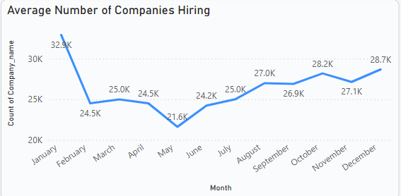
Insight:The visual indicates that most companies begin hiring from October, peaking in January. In October, 28.2k companies were hiring, followed by a slight dip to 27.1k in November. Hiring activity then increased significantly, reaching 32.9k companies in January. After January, hiring declined to 24.5k in February and remained relatively stable for a few months before dropping further to 21.6k in May. It then gradually increased again leading up to the following January
5. Top 3 Demanded Job Fields Each Year
A matrix table was created to display the top 3 in-demand job fields for each year. This enables the company to align hiring strategies with industry demand and growth sectors.
Top3_demanded_job =
VAR selected_year = SELECTEDVALUE('bidb job_postings1'[Job_posting_date].[Year])
VAR on_demand_jobs =
    TOPN(3,
         SUMMARIZE(
             FILTER('bidb job_postings1',
                    'bidb job_postings1'[Job_posting_date].[Year] = selected_year &&
                    'bidb job_postings1'[Job_field] <> "No Clear Specifications"),
             'bidb job_postings1'[Job_field],
             "count_job_field", COUNT('bidb job_postings1'[Job_field])
         ),
         [count_job_field], DESC)
RETURN CONCATENATEX(on_demand_jobs, 'bidb job_postings1'[Job_field], ", ")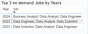
Insight:Based on the data provided, the top three in-demand jobs in 2022 and 2023 were consistently Data Engineer, Data Analyst, and Data Scientist. However, in 2024, Business Analyst replaced Data Scientist in the top three. The order of the data in each row reflects the ranking order, showing the top 1st, 2nd, and 3rd positions for each year.
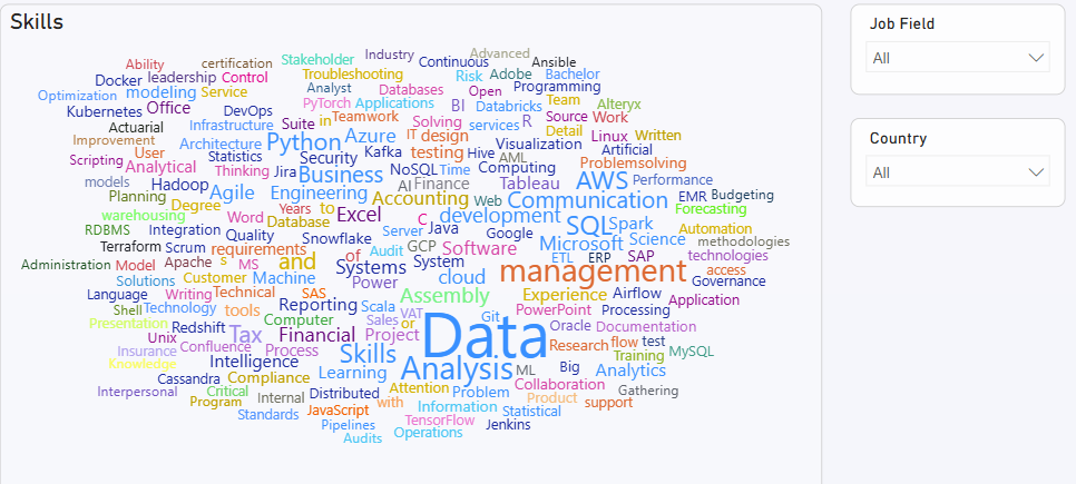
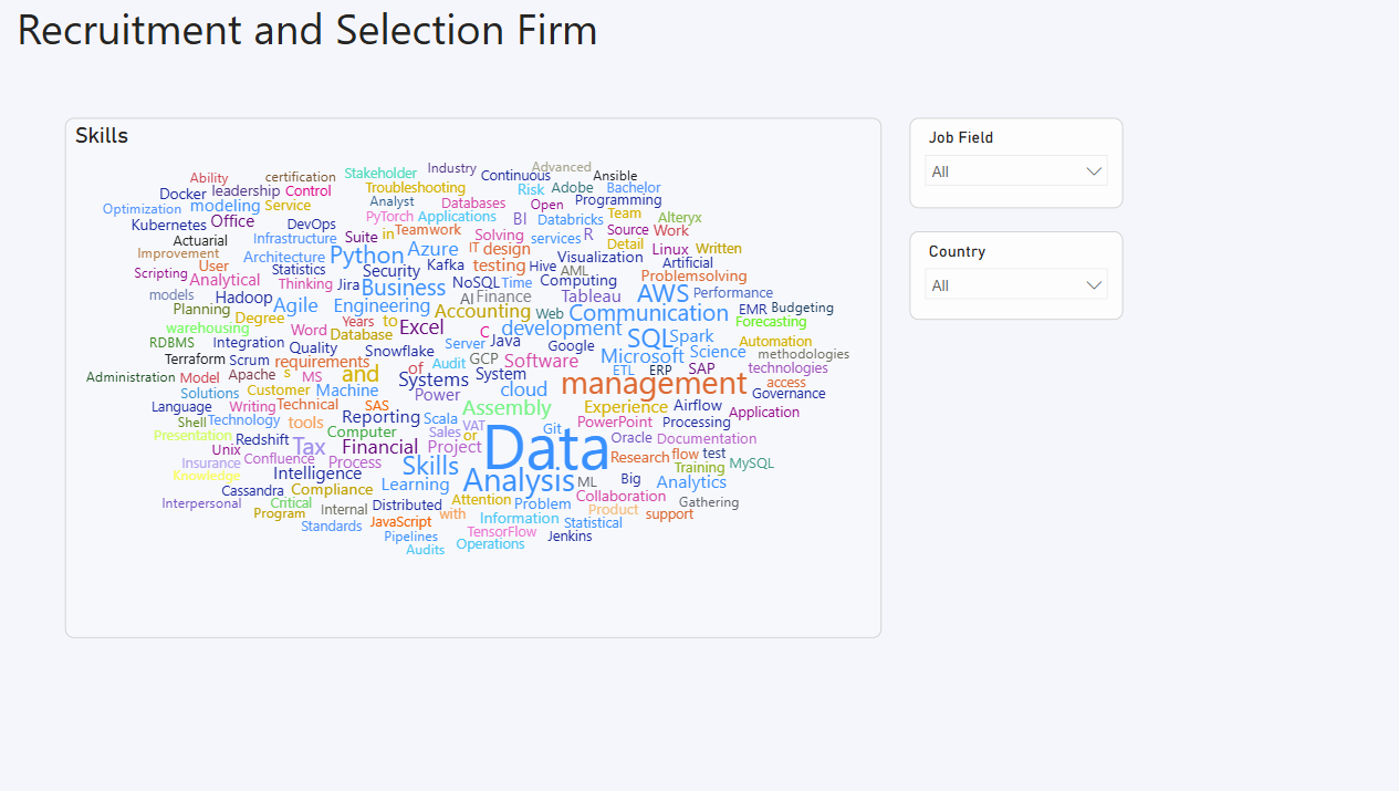
6. Most In-Demand Skills
A word cloud was implemented using the Job_skills column to visualize the most frequently required skills across postings. This helps stakeholders prioritize workforce development and training aligned with current market needs.
4. Final Dashboard
Technology Stack
- Python: pandas, SQLAlchemy for ETL
- MySQL: Central data repository
- Power BI: DAX measures, Power Query, Visualizations
- Performance Optimization: Aggregations, Columnar storage